TB 26-08 Complex Modes in Lightly Damped Structural Systems: A Two-Mode Interaction Perspective

For more information, contact Joel W. Sills, Langley Research Center, [email protected]

Download the PDF version

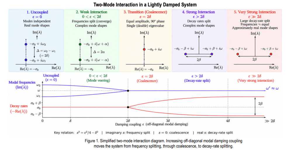
Complex mode shapes can emerge in a linear structure even when overall damping is low. This behavior can occur when two structural modes are closely spaced in frequency and are coupled through nonproportional damping. As the damping interaction increases, the two modal frequencies move toward one another while the mode shapes become increasingly complex. At a critical interaction level, the two frequencies coalesce. Beyond this point, the frequencies remain approximately equal while the modal decay rates separate. At very strong interaction, the mode shapes become approximately real again, but as different combinations of the original uncoupled modes. This framework provides a simple physical interpretation of mode veering, complex mode formation, eigenvalue coalescence, and decay-rate splitting in lightly damped structural systems.

Why Complex Modes Can Appear at Low Damping
Classical modal analysis often treats lightly damped structures as nearly proportional systems with real mode shapes. That interpretation can become misleading when two modes are closely spaced. In modal coordinates, nonproportional damping introduces an off-diagonal coupling term ε. The relevant question is therefore not simply whether damping is small, but whether the coupling is large relative to the baseline half-frequency separation δ=(ω2 -ω1 )/2.

Reduced Perturbation Framework
For a closely spaced pair, define the central eigenvalue λ0 ≈-ζω +iω and write the coupled eigenvalues as λ1,2=λ0 ±s. Under lightdamping and close-mode asymptotic assumptions, the local quartic eigenvalue problem reduces to s²=ε²/4-δ². This single relation determines the direction of eigenvalue separation in the complex plane, as summarized in Figure. 1. For 0<ε 2δ, s = ±β and the split is predominantly horizontal (decay rate). As ε increases further, β increases and the two decay rates separate more strongly while their frequencies remain approximately equal.

Engineering Interpretation and Recommended Practice
Complexity in an identified mode shape should not automatically be interpreted as evidence of heavy damping, nonlinearity, or poor test data. For a close modal pair, examine the complex poles together with mode-shape phase. Frequency convergence accompanied by near-quadrature modal components is consistent with the imaginary-s regime; nearly equal frequencies accompanied by decay-rate separation is consistent with the real-s regime. The framework also provides a practical testanalysis bridge: s=(λ1 -λ2 )/2 can be obtained from identified poles, while δ can be estimated from the uncoupled or pretest analytical modal spacing. These quantities can then be used to estimate the effective interaction strength and determine proximity to the transition boundary.
References

1. Majed, A., Henkel, E. E., and Sills, J. W., Emergence of Complex Modes in Lightly Damped Structural Systems: A Reduced Perturbation Framework, NASA/TM-20260007553, August 2026.

Source: www.nasa.gov
Voyager Technologies’ Griffin-1 Completes Environmental Testing at NASA JPL

3 Min Read

Voyager Technologies’ Griffin-1 Completes Environmental Testing at NASA JPL

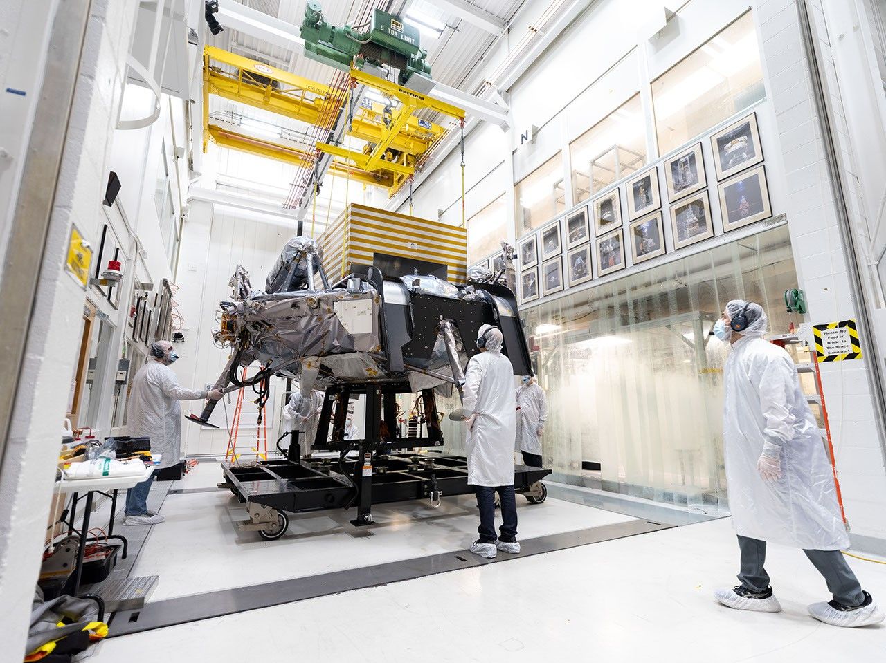
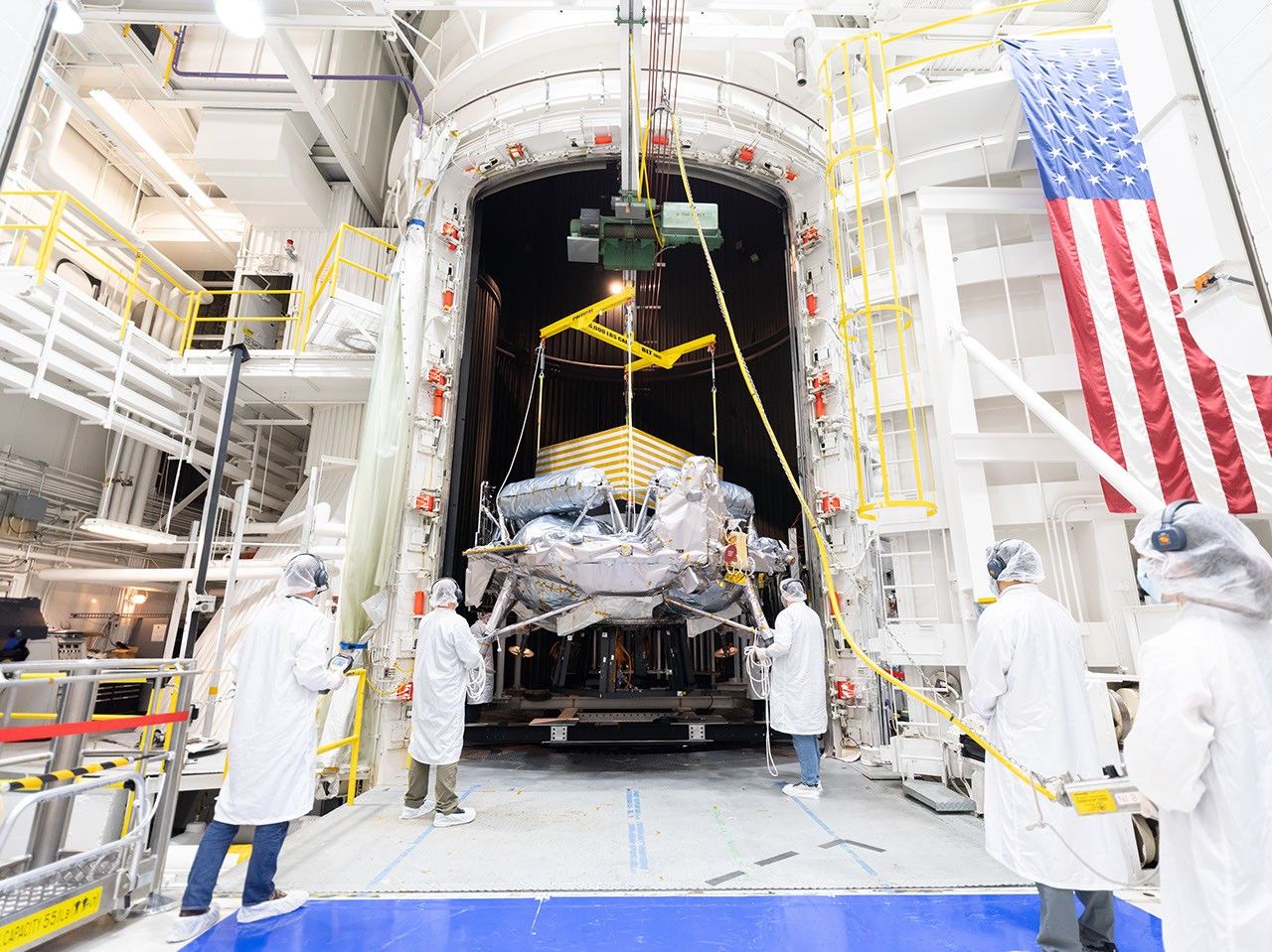
Engineers in white clean-room garb and hairnets guide a spacecraft suspended from a crane into a large thermal vacuum chamber inside a high-bay facility with an American flag hanging on the wall.

PIA26708

Credits:
NASA/JPL-Caltech

Description

A lunar lander from Voyager Technologies completed nearly three months of environmental testing at NASA’s Jet Propulsion Laboratory in Southern California in late September 2026. The tests demonstrate that the spacecraft is prepared to face the harsh conditions of launch, its journey to the Moon, and landing on the surface. Its final trial was in JPL’s historic 25-Foot Space Simulator, a thermal vacuum chamber listed on the National Register of Historic Places for its role in supporting historic missions like those of the Ranger, Surveyor, Mariner, and Voyager programs. 

Engineers and technicians on Aug. 31, 2026, used a crane to position the spacecraft within the towering chamber, where Griffin-1 alternately baked at up to 167 degrees Fahrenheit (75 degrees Celsius) and froze at temperatures as low as minus 148 F (minus 100 C). This thermal vacuum testing simulates the extreme temperatures the spacecraft will experience during its mission. The yellow-striped box atop the lander simulates a payload that will later be attached to the spacecraft: Astrolab’s FLIP (FLEX Lunar Innovation Platform) rover.

Engineers in white clean-room garb monitor a large spacecraft as it is hoisted by a yellow overhead crane in a hallway in a bright, high-tech laboratory. Framed photos line both sides of the hallway.
Figure A

In Figure A, engineers and technicians move Griffin-1 through a hallway leading to the 25-Foot Space Simulator on Aug. 31. The corridor is lined with photographs of some of the historic spacecraft that have been tested in the facility since the 1960s.

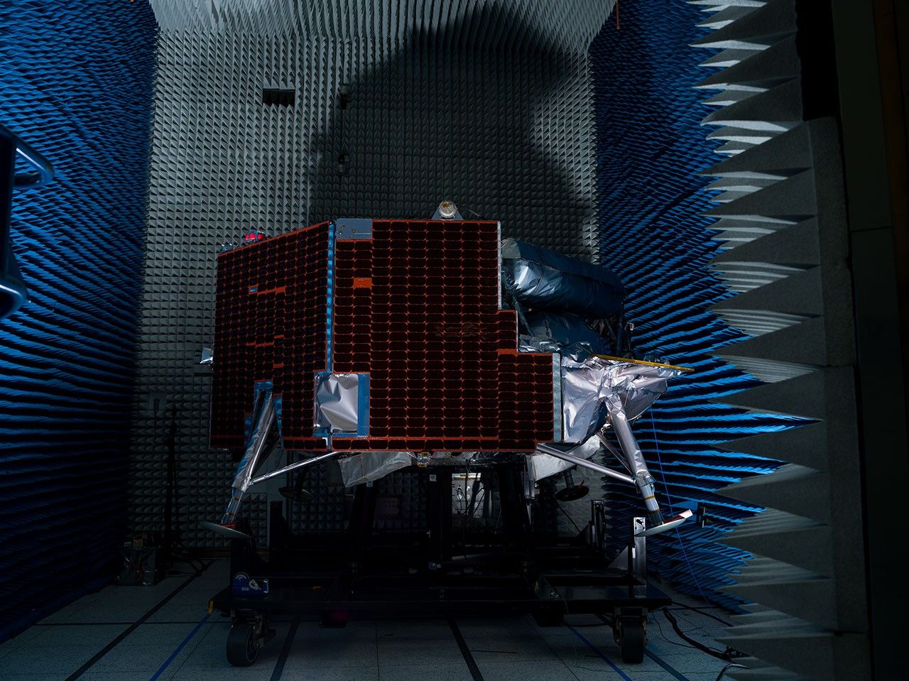
A lunar lander equipped with dark solar panels and foil-wrapped legs sits on a platform inside a dark anechoic chamber lined with blue and gray foam spikes.
Figure B

Figure B shows Griffin-1 on July 29 in an anechoic chamber for electromagnetic interference and electromagnetic compatibility testing, which ensures signals from the spacecraft’s electronic components don’t interfere with one another. Long foam spikes line the chamber walls to absorb sound waves and electromagnetic waves.

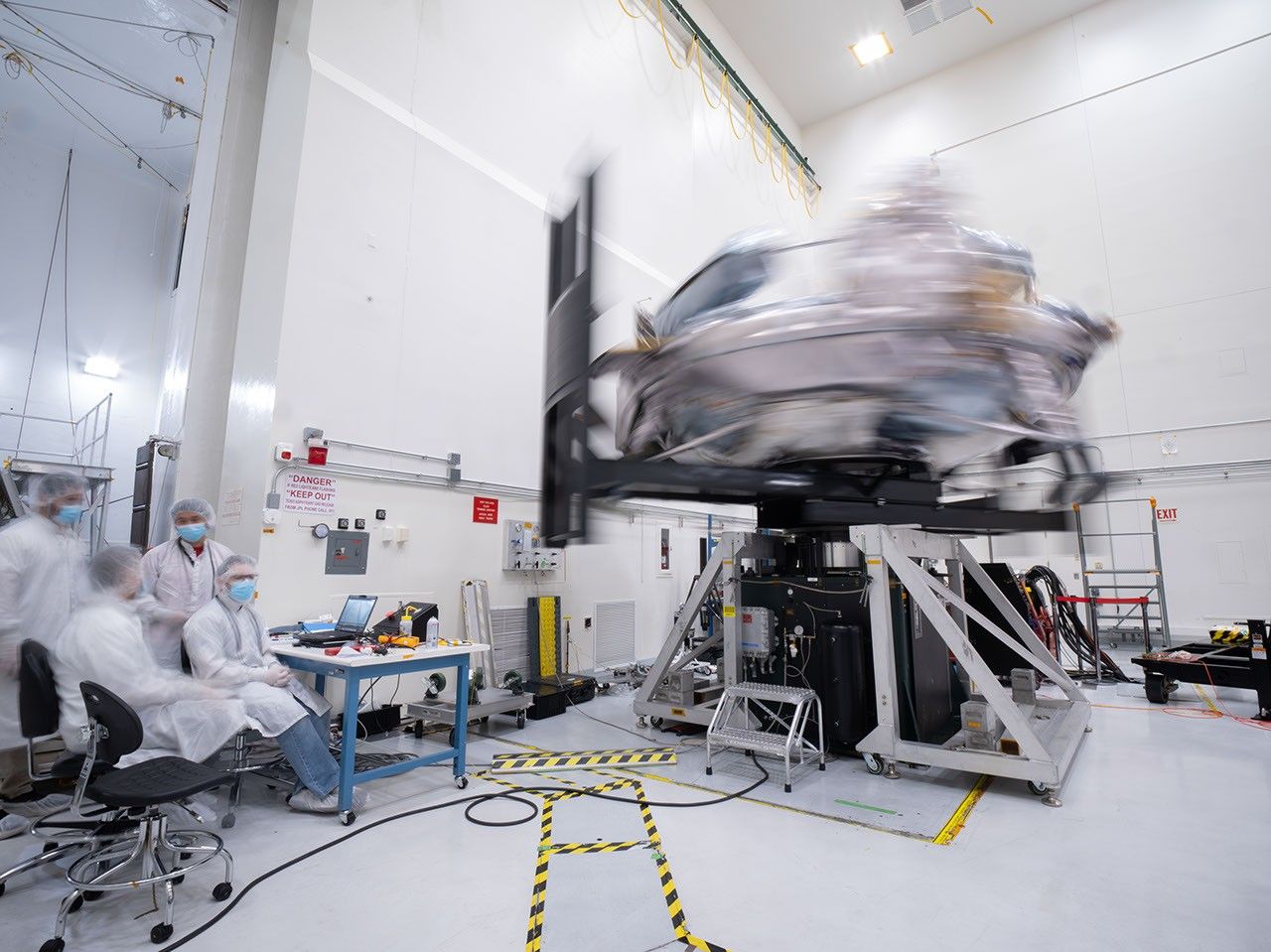
Engineers in white clean-room frocks monitor a silvery spacecraft spinning so rapidly it’s blurred on a test rig inside a bright laboratory.
Figure C

In Figure C, taken on July 20, Griffin-1 rotates rapidly on a special table to measure its mass properties, enabling engineers to look for any unexpected wobbles as they assess how the vehicle will move through space — vital information for determining the spacecraft’s readiness for flight and surface operations.

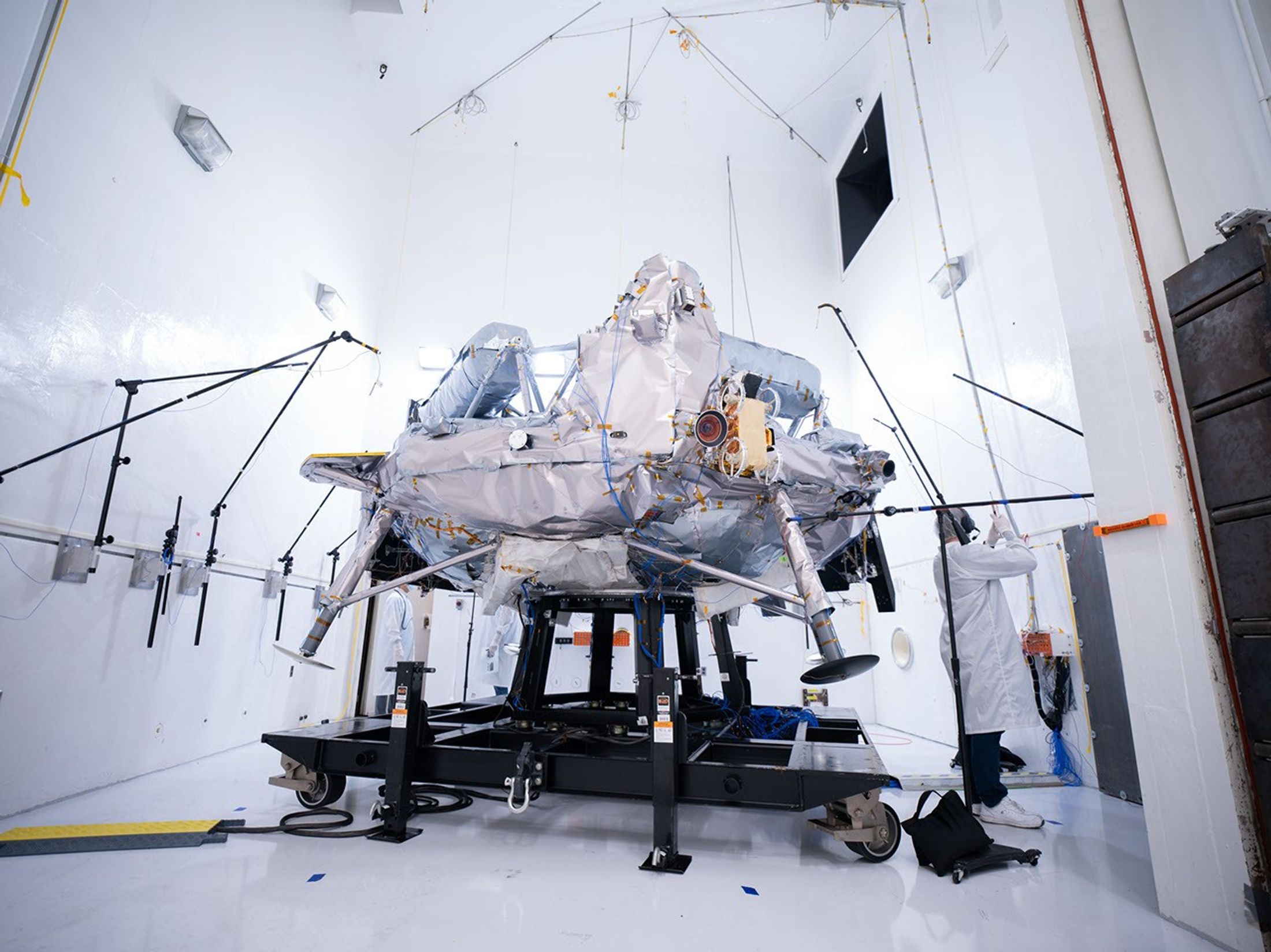
A silvery spacecraft sits on a test frame surrounded by microphones and testing equipment inside a bright white acoustic test chamber, while an engineer in a lab coat works nearby.
Figure D

In Figure D, microphones are arrayed around Griffin-1 on Aug. 12 during acoustic testing in which giant horns powered by compressed gaseous nitrogen blast the spacecraft with up to 153 decibels inside the sealed acoustic chamber to mimic the roar of launch. 

Griffin-1 also endured vibration testing, during which hundreds of sensors monitored the spacecraft as a “shaker table” rattled it in three directions — with increasingly intense force — to simulate the ride out of Earth’s atmosphere atop a rocket.

After proving its mettle at JPL, Griffin-1 was shipped back across the country to Voyager Lunar Systems’ Pittsburgh facility for final assembly. Part of NASA’s CLPS (Commercial Lunar Payload Services) initiative within the Moon Base Program, Griffin-1 is expected to launch in late 2026 aboard a SpaceX Falcon Heavy rocket. The infrastructure-class lander will deliver more than 1,100 pounds (455 kilograms) of cargo — 10 payloads from six countries — to Nobile Crater near the lunar South Pole.

Caltech in Pasadena, California, manages JPL for NASA.

Source: science.nasa.gov

Transporter-18 SmallSats Encapsulation

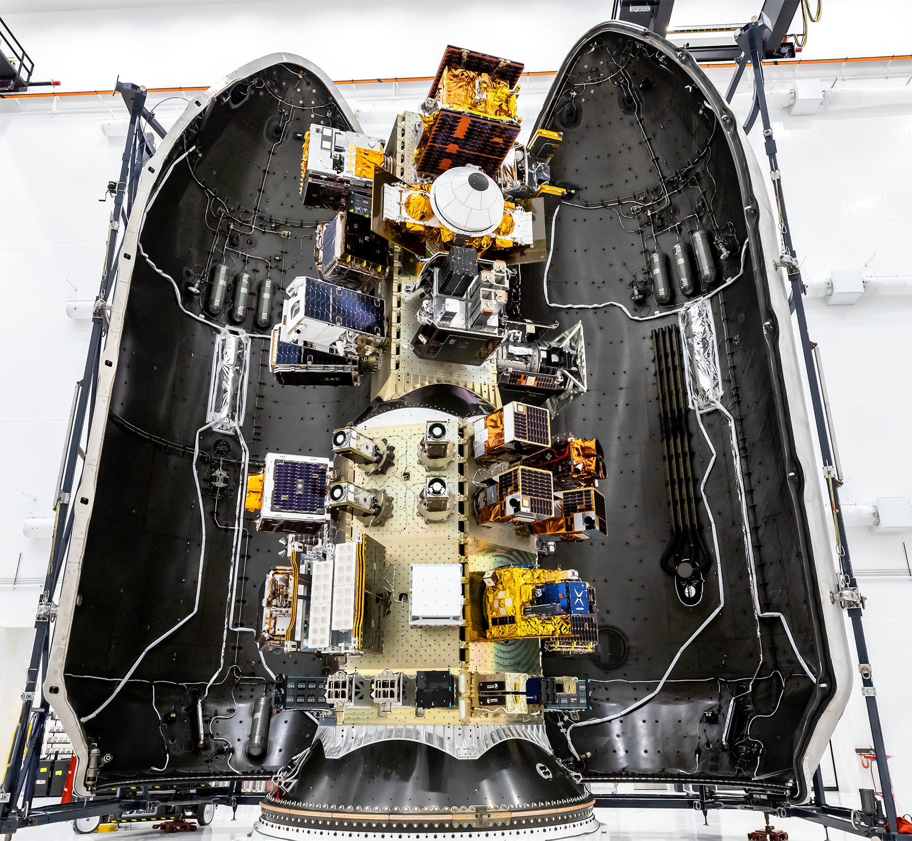
View of a SpaceX payload fairing interior showing mounted satellites and hardware arranged along the center structure, surrounded by the curved black fairing walls.
SpaceX

Three NASA-supported small spacecraft, along with many commercial payloads, are shown before being encapsulated in a SpaceX Falcon 9 ahead of launch on Oct. 1, 2026. The ASCENT Propulsion Dual Mode CubeSat, the Supernova Remnants and Proxies for ReIonization Testbed Experiment (SPRITE) CubeSat, and the Small Spacecraft Propulsion and Inspection Capability (SSPICY) mission will demonstrate new propulsion technologies, study how galactic dust and high-energy radiation move through galaxies, and advance capabilities for inspecting inactive satellites.

Image credit: SpaceX

Source: www.nasa.gov
Perseverance Navcam Image Marks Record Drive

1 Min Read

Perseverance Navcam Image Marks Record Drive

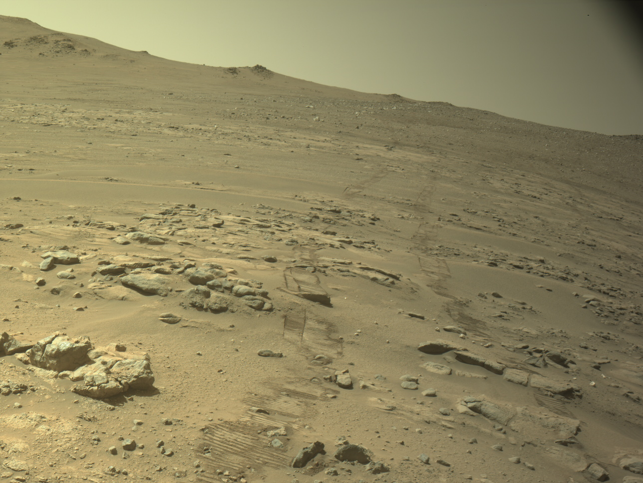
Rover tracks press into the sand of a rocky, sloping Martian landscape, leading upward toward a distant ridge under a pale, hazy sky.

PIA26812

Credits:
NASA/JPL-Caltech

Description

Rover tracks and a rocky Martian landscape are shown in this image captured by one of the navigation cameras (navcams) aboard NASA’s Perseverance Mars rover on Oct. 11, 2026, the 2,006th Martian day, or sol, of the mission. During that sol’s drive, spanning 299.6 feet (91.31 meters), the mission passed a major milestone: pushing Perseverance’s total driving distance beyond that of the agency’s Opportunity rover, which logged 28.06 miles (45.16 kilometers) during its 15-year mission on Mars.

NASA’s Jet Propulsion Laboratory, which is managed for the agency by Caltech in Pasadena, California, built and manages operations of the Perseverance rover on behalf of the agency’s Science Mission Directorate in Washington, as part of NASA’s Mars Exploration Program portfolio.

For more about Perseverance: https://science.nasa.gov/mission/mars-2020-perseverance/

Source: science.nasa.gov

NASA’s Record-Setting Perseverance Rover Team

1 Min Read

NASA’s Record-Setting Perseverance Rover Team

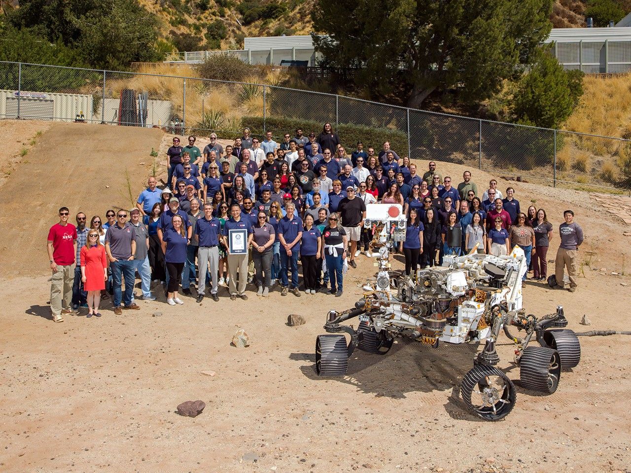
About 100 members of NASA’s Perseverance Mars rover mission team stand posed together in a sandy outdoor test facility alongside a full-scale Mars rover model.

PIA26813

Credits:
NASA/JPL-Caltech

Description

Members of NASA’s Perseverance Mars mission team gather in the Mars Yard at the agency’s Jet Propulsion Laboratory in Southern California with a certificate from Guinness World Records marking the rover distance record on the Red Planet. Positioned in front of the team is OPTIMISM (Operational Perseverance Twin for Integration of Mechanisms and Instruments Sent to Mars), a full-scale engineering model used to plan the rover’s driving routes and science activities on Mars. NASA JPL, which is managed by Caltech, built and manages operations of the Perseverance rover on behalf of the agency’s Science Mission Directorate in Washington, as part of NASA’s Mars Exploration Program portfolio.

For more about Perseverance: https://science.nasa.gov/mission/mars-2020-perseverance/

Source: science.nasa.gov
Comparing Off-World Rover Driving Distances

1 Min Read

Comparing Off-World Rover Driving Distances

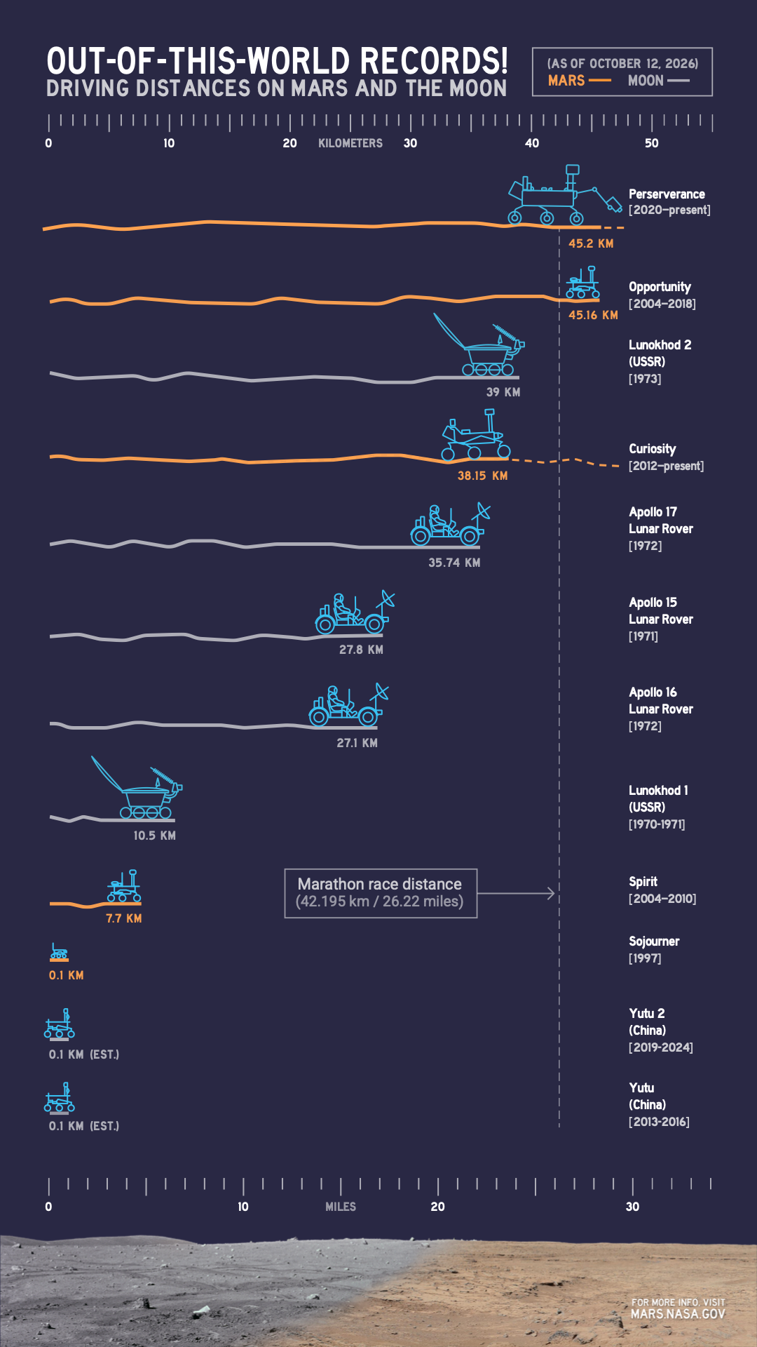
An infographic compares driving distances on Mars and the Moon by various rovers, with NASA’s Perseverance leading as of Oct. 11, 2026, at more than 45 kilometers.

PIA26814

Credits:
NASA/JPL-Caltech

Description

This infographic illustrates the distances driven by various rovers on the surface of Earth’s Moon and Mars. Of the vehicles shown, the NASA Mars rovers Perseverance and Curiosity are still operational and moving across the surface; the figures shown for those two are distances driven as of Oct. 11, 2026. As of that date, Perseverance exceeded the distance record held by NASA’s Opportunity rover, which came to a final halt in 2018 at about 28.1 miles (45.16 kilometers) driven. 

NASA’s Jet Propulsion Laboratory, which is managed for NASA by Caltech in Pasadena, California, built and manages operations of the Perseverance rover on behalf of the agency’s Science Mission Directorate in Washington, as part of NASA’s Mars Exploration Program portfolio.

For more about Perseverance: https://science.nasa.gov/mission/mars-2020-perseverance/

Source: science.nasa.gov

Antarctic Sea Ice Grows to Its 2026 Maximum

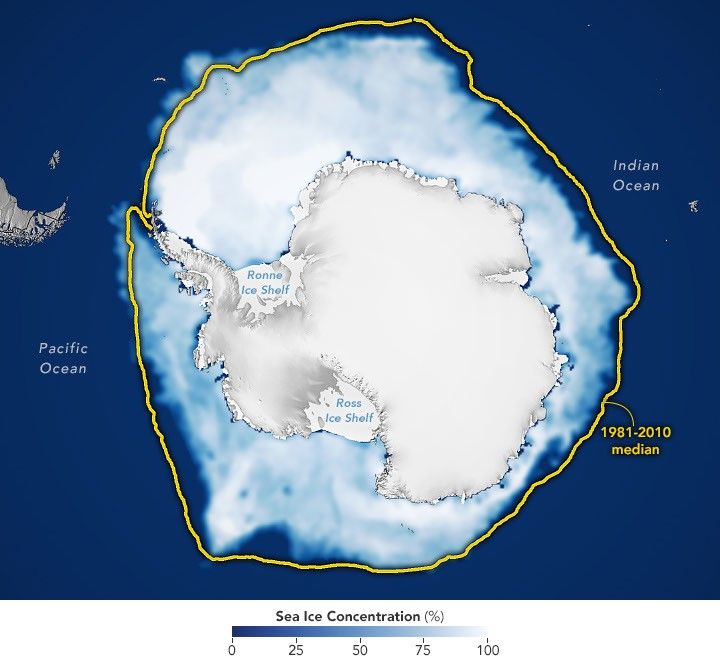
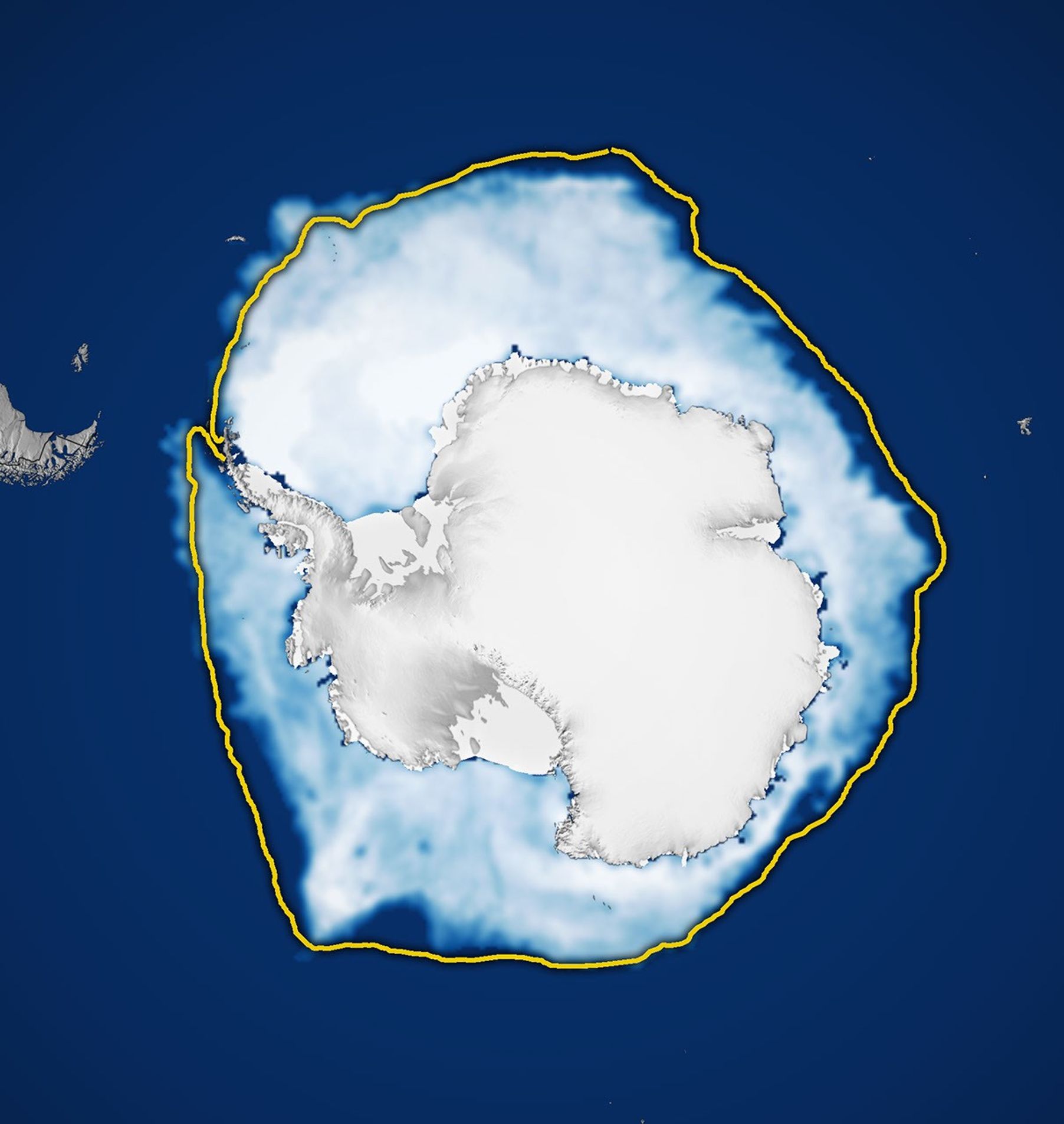
A map shows white Antarctic sea ice on September 14, 2026, the day it reached its annual maximum extent. The 1981–2010 median is outlined in yellow.
Antarctic sea ice reached its annual maximum extent on September 14, 2026—the third-lowest maximum in the satellite record.
NASA Earth Observatory/Michala Garrison

This story is an update to the Antarctic sea ice feature in our World of Change series tracking long-term change on Earth’s surface through satellite imagery.

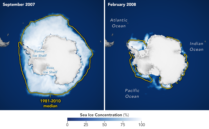
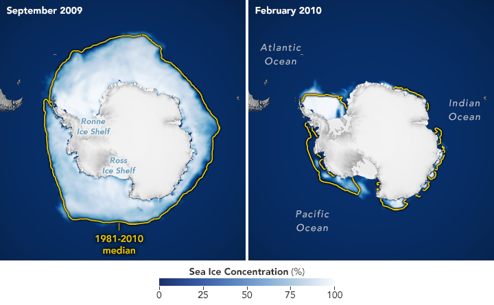
Unlike the Arctic—an ocean basin surrounded by land—the Antarctic is a large continent surrounded by an ocean. Because of this geography, sea ice has more room to expand during the winter. However, that ice also stretches into warmer latitudes, leading to more melting in the summer. Antarctic sea ice usually peaks in September, around the end of the Southern Hemisphere’s winter, and retreats to a minimum in February.

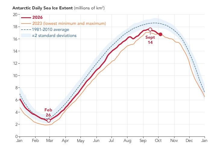
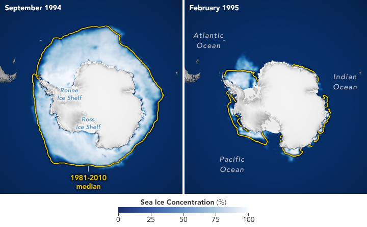
According to NASA and the National Snow and Ice Data Center (NSIDC), Antarctic sea ice in 2026 likely reached its annual maximum extent on September 14 (above). On that date, the ice covered an estimated 17.59 million square kilometers (6.79 million square miles), making it the third-lowest maximum on record.

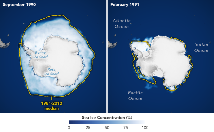
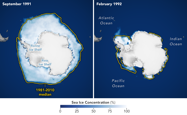
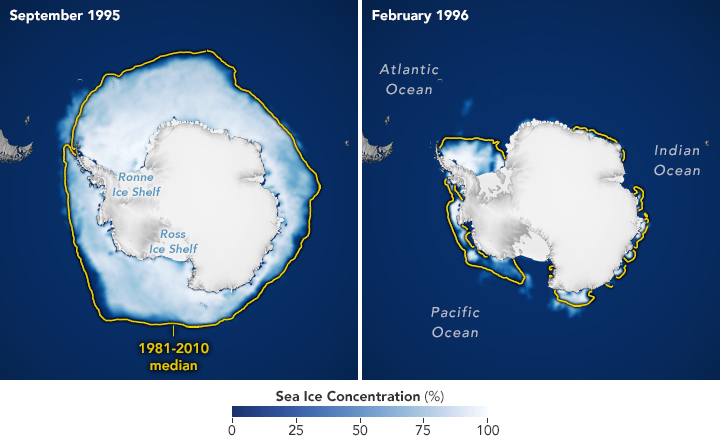
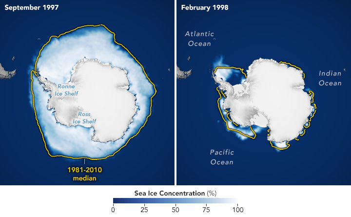
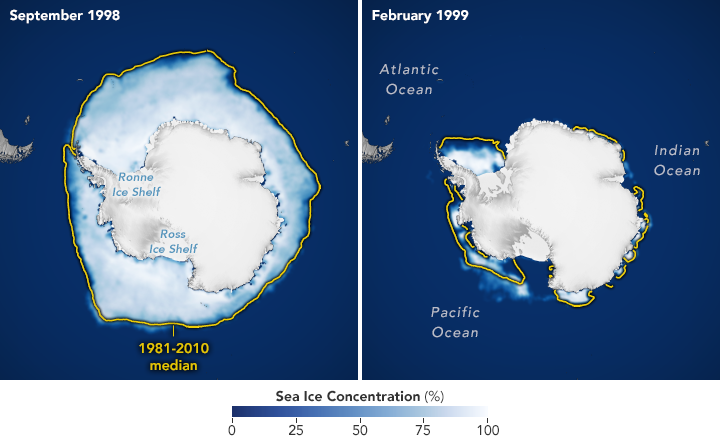
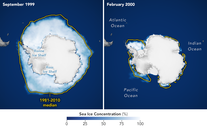
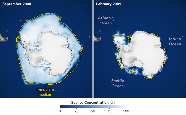
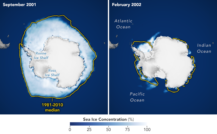
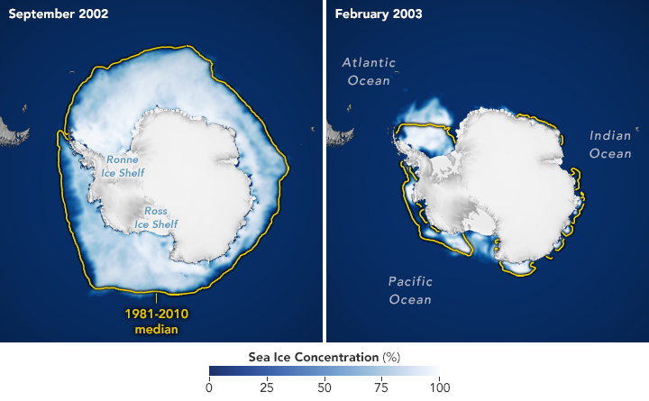
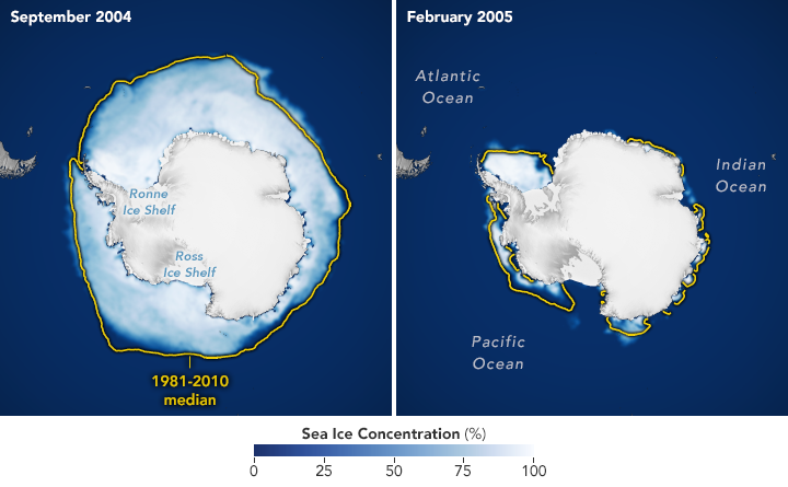
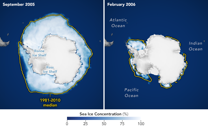
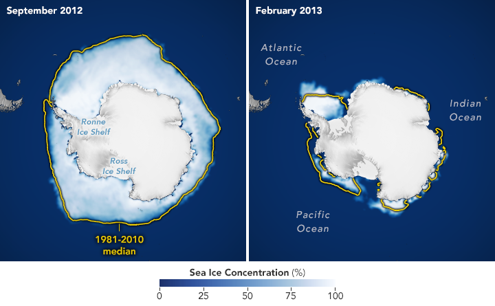
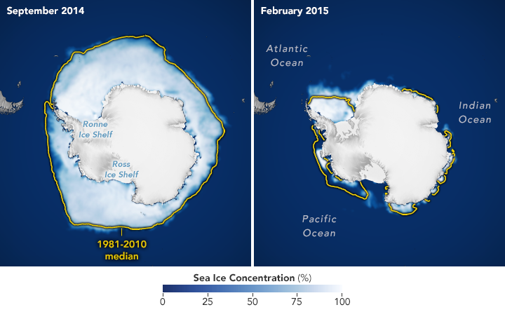
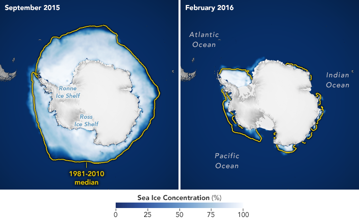
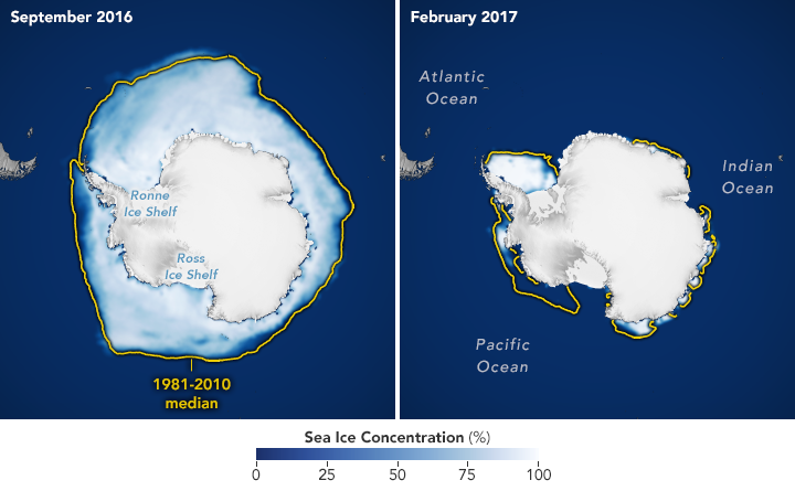
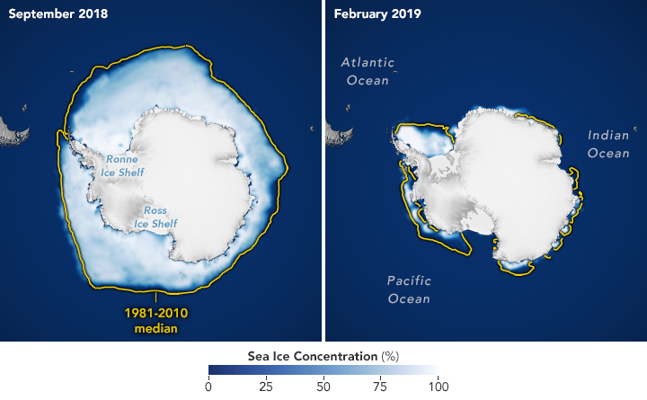
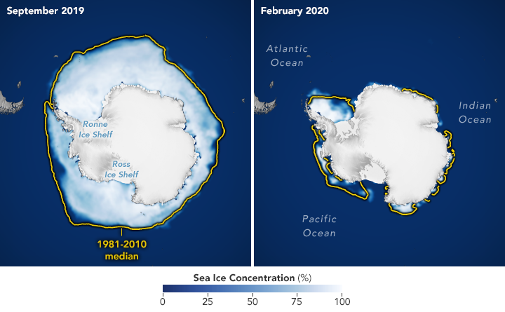
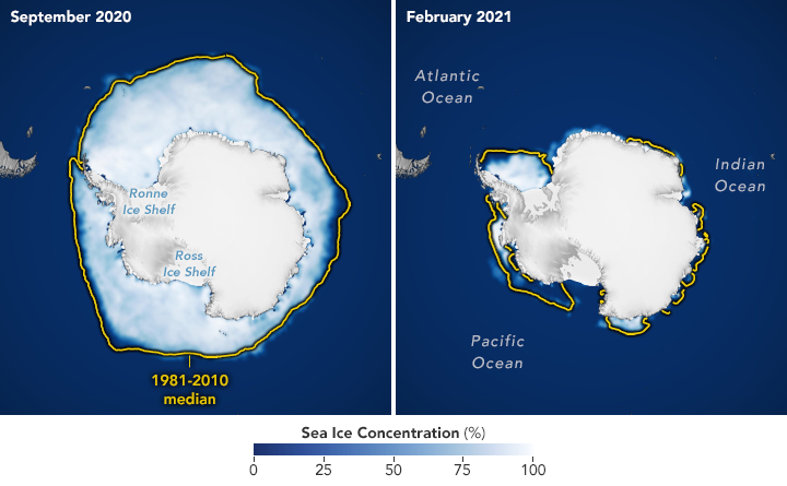
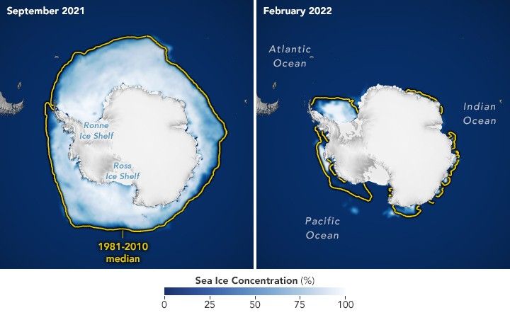
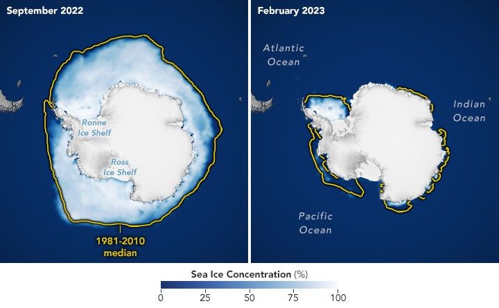
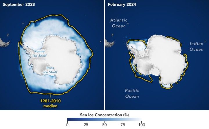
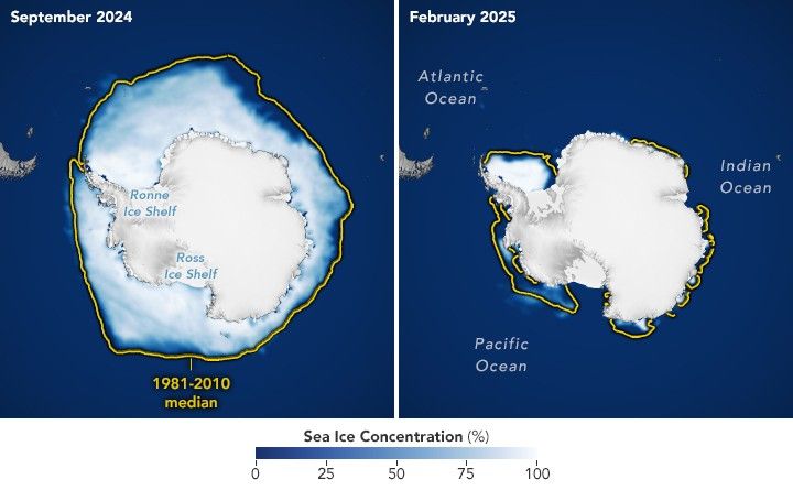
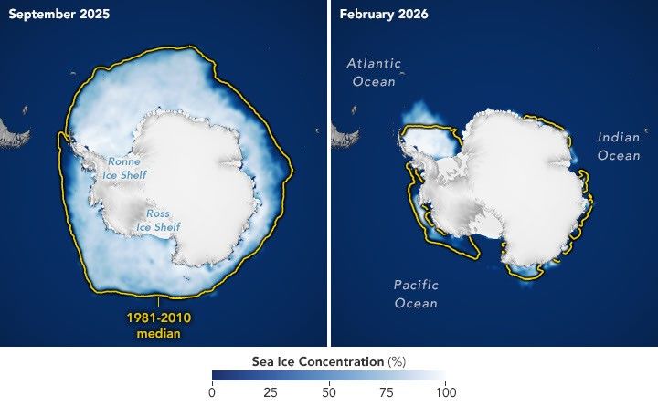
The maps below show the average concentration of Antarctic sea ice for the month of September (left) and the following February (right) from 1990 to 2026. Opaque white areas indicate the highest concentrations, and dark blue areas are open water. The images include only areas where ice concentration was at least 15 percent, a threshold scientists commonly use to count an area as ice-covered in satellite data. Scientists refer to the total area of these regions as the “sea ice extent.”

From Record Highs to Record Lows

From 1979 until 2014, total Antarctic sea ice increased by about 1 percent per decade. Whether the increase was a sign of meaningful change is uncertain because ice extents vary considerably from year to year around Antarctica. For three consecutive years, from 2012 to 2014, satellites observed new record highs for winter sea ice extent. These highs occurred while Arctic ice was in steep decline.

The climb came to an end in 2015, and significant decreases in sea ice around Antarctica started to occur in 2016. There have since been years with small rebounds, but overall, Antarctic sea ice coverage has largely remained lower than normal. Both the record low minimum and record low maximum occurred in 2023. Scientists will continue to observe the area each year to find out if the decline is part of a long-term change or a statistical fluctuation.

A line chart of Antarctic sea ice extent shows the 1981–2010 average as a blue dashed line, 2023 (the lowest minimum and lowest maximum on record) in orange, and 2026 in red.

Seeing Through the Clouds

To determine sea ice extent, scientists rely on satellites with passive microwave sensors that measure the microwave energy Earth naturally emits. Sea ice emits more of this energy than open water, so it stands out in microwave images. Because microwaves pass through clouds, the satellites can observe sea ice regularly, regardless of weather.

The record began in late 1978 with data collected by NASA’s Nimbus-7, followed by Defense Meteorological Satellite Program (DMSP) satellites starting in 1987, and by NASA’s Aqua satellite between 2002 and 2011. In 2025, scientists began using observations from the Japan Aerospace Exploration Agency’s GCOM-W satellite. 

NASA Earth Observatory images by Michala Garrison, using data from the National Snow and Ice Data Center.

References & Resources

You may also be interested in:

Stay up-to-date with the latest content from NASA as we explore the universe and discover more about our home planet.

Arctic Sea Ice Shrinks to Its 2026 Minimum

4 min read

Satellite records show Arctic sea ice covering less of the ocean in both winter and summer.

Article

A Changing World for Emperor Penguins

7 min read

Experts are analyzing decades of images from Landsat satellites for clues about how the iconic birds have responded to sea…

Article

Pink Penguin Guano Provides Diet Clues

3 min read

The color of Adélie penguin droppings reveals what the birds are eating, offering scientists a way to track how sea…

Article

Source: science.nasa.gov
APOD: 2026 October 12 – Jupiter and the Moons

APOD

Astronomy Picture of the Day

Discover the cosmos! Each day a different image or photograph of our fascinating universe is featured, along with a brief explanation written by a professional astronomer.

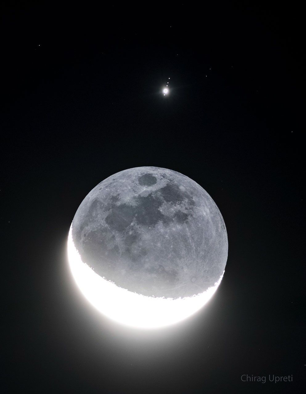
In front of a dark background an image of Earth's Moon  appears with a lower crescent brightly lit. The rest of the Moon is also faintly visible. Above the Moon is a bright point of  light surrounded by four fainter points of light in row. Please see the explanation for more detailed information.

Jupiter and the Moons

Explanation: How many moons can you see? The best answer is five: four orbiting Jupiter and Luna orbiting Earth. This multi-moon picture was possible because Earth’s Moon moved directly in front of Jupiter last week. The featured image is a series of exposures near alignment taken from Westchester, New York, USA. The sunlit crescent of Earth’s Moon, on the lower left, is overexposed, while the Moon’s night side, on the upper right, is faintly illuminated by Earthshine. Lined up nearly vertically above our Moon, listed from bottom to top, are Jupiter’s bright Galilean satellites: Ganymede, Io, Callisto, and Europa. Callisto, Ganymede, and Io are larger than Earth’s Moon, while Europa is only slightly smaller. NASA’s robotic spacecraft Juno is currently orbiting Jupiter and has made close passes near three of these moons.

Tomorrow’s picture: stairway to heaven

Date: October 12, 2026
Credit & Copyright: Chirag Upreti
Authors & editors: Robert Nemiroff, Jerry Bonnell, Cecilia Chirenti, Keighley Rockcliffe
A service of: ASD at NASA / GSFC,
NASA Science Activation & Michigan Tech. U.

Source: science.nasa.gov